Utility is ultimate yardstick of evaluating any theory. Therefore, different theorists criticize their predecessors and present new theories to increase their utility. Similarly, D.M. Smith’s theory of industrial location tries to help an entrepreneur in determining a profitable location for satisfying the needs of the firm. He published his ideas about location of industries in his book titled “Industrial Location: An Economic Geographical Analysis (1966)”.
Smith’s Basic Idea
Basically, Smith’s ideas originate from Herbert Simon’s Theory of Satisficing. Simon opines that all producers do not have complete knowledge of the ground realities, therefore, they can not make perfect decision to maximize profit. Instead, they settle at a cost-price ratio which satisfies the expectations of the producers. Smith applied this idea in context of geographical space to choose a location where the minimum needs and objectives of the firms are satisfied. Based on imperfect knowledge, some producers will make more profit while some less. So, there is a spatial margin of profitability within which firms can remain profitable. Outside this margin, the firms will ultimately go bankrupt. Unlike Weber’s Industrial Location Theory, Smith believes that there are more than one optimum location in a given area.
Assumptions
Smith made following assumed certain conditions for working of his theory as follows.
- Producers have imperfect knowledge of spatial variation of cost and revenue.
- The sources of input factors such as land labor and capital is fixed, geographically. They are distributed unevenly over space.
- The supply of factors of production is unlimited.
- Producers are rational people.
- Demand of the goods and services is constant but not same at various locations of production. It means that the demand may vary over space but it remains constant over time.
- Given the above conditions, the producer tries to locate his firms at a profitable location which satisfies him.
- Industrial agglomeration are not always the location which satisfies the producers but some producers may locate there for maximum profit.
Working of Smith’s Industrial Location Theory
Inititally, Smith tried to find the least cost location like Weber’s Industrial Location Theory by using isodapanes. He soon realized that it is not a practical theory. So, he inculcated some real world assumptions in his theory e.g. imperfect knowledge, need for satisfying level of profit etc. to make it more practical. However, he used isopleths like weber did. In pursuit of determining such locations, Smith uses Cost Contours and Revenue contours which represent lines joining areas of equal cost and revenue respectively. By using these isopleths, he drew cost and revenue curves representing variation in cost and revenue over space. That is why this theory is also called Area-Cost Curve Theory. Smith outlined three cases of industrial location. Let us discuss these cases in detail.
1. Constant Cost-Variable Revenue
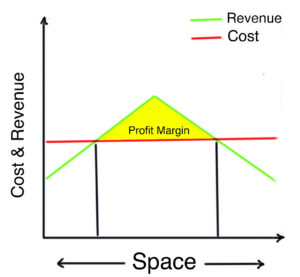
In this case, the cost of production remains constant over space while the revenue changes. So, the only way to increase profit is by increasing the sale of the goods. In real world, the demand exists unevenly over space. The large urban centers have the highest demand and it decreases outwards towards the rural areas. In such scenario, the producer may locate anywhere at a location where the revenue exceeds the cost. The zone between the points where the cost becomes equal to revenue is spatial margin of profitability (See Fig. 1)
For example, The National Capital Region of Delhi has highest population and has the highest level of demand which decreases outwards. The revenue may be highest in the center and decreases towards peri-urban areas.
2. Variable Cost-Constant Revenue
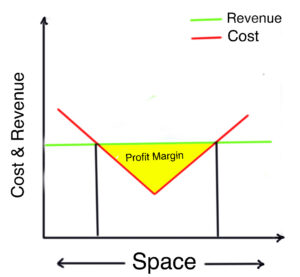
In this case, the cost is variable but the revenues is constant over space. Usually, some physical and economic factors may lead to variable cost. For example, the cost of producing a weight loosing product will decline towards the source of a raw material and will be minimum at source e.g. for iron and steel industry. It is so because the source location has the loading and unloading facilities along with lowest transportation cost as Hoover suggested. The only option to increase profit is by reducing cost as the revenue is constant over space. Ultimately, the firm has to locate it’s business within a spatial margin.
3. Variable Cost-Variable Revenue
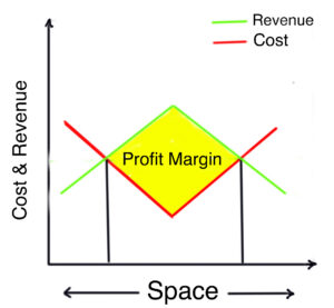
In real world, the cost and revenue for most products vary over space. The consumer buys from the products having the lowest price among it’s competitors. As a producer, one can reduce price only if the cost is low and the revenue is high. Hence, producer will be able to locate his firm within a spatial limit where price exceeds the cost. Larger the difference, larger will be the ability of producer to adjust price. Given all this, consumer will not always go at location of lowest price because transportation cost will increase the final price. Hence, producers within the spatial limit will be able to survive. Outside the limit, the firms will ultimately go bankrupt.
Conclusion
To summarize, we can argue that Smith shines among his peers in determining the a profitable location for industry. He understands the the location of maximum profit is not always desirable due to various practical reasons such as limitation of space, overcrowding, inflation of rent etc. Hence, the producers locate at a different location within the margin which satisfies him or the needs of the firm. Smith explains the geographical decision making through behavioral approach while keeping the economic rationale intact. His ideas accommodates the ideas of Weber, Perroux’s Growth Pole Theory and Hoover’s Theory of Industrial Location while contributing a new theme to the problem of industrial location.
Kulwinder Singh is an alumni of Jawaharlal Nehru University, New Delhi and working as Assistant Professor of Geography at Pt. C.L.S. Government College, Kurukshetra University. He is a passionate teacher and avid learner.