Alfred Weber is considered one of the pioneers of locational analysis in Geography. He gave his theory of industrial location in 1909. Weber’s theory of industrial location is a beautiful example of combining economic parameters with spatial parameters to arrive at a profitable location for industries. It is also known as Least Cost Theory because this theory tries to find a location of least cost for an industrial location.
Basic Idea of Industrial Location Theory
- Basically, the theory of industrial location tries to arrive at a location of least cost for industrial operations.
- Weber used some economic and spatial parameters which determine the cost of products e.g. transport cost, labor cost, agglomeration effect etc.
- According to Weber, transport cost is an overarching factor in determining the market price of a product. Hence, the location with least transport cost is the optimum location.
Assumptions of Industrial Location Theory
Like any other economic theory, Industrial Location Theory needs certain conditions for its application. In the real world such conditions do not exist perfectly. Therefore, Weber made the following assumptions.
- Isotropic Surface: Weber assumed that geographic space is plain and does not have topographic undulations because transport cost varies over different types of landscape.
- Ubiquitous and Fixed Raw Materials: The sources of raw material are evenly distributed and have fixed location.
- Constant Labor Supply: The wages of workers are constant over geographic space. It does not change from one place to another, however the wage rate varies from one place to another.
- Immobile Labor-force: The workers do not migrate from one place to another. Therefore, the supply of labor in a given point in time remains constant over space.
- Transport Cost Increases Uniformly: The transport cost rises with increasing distance and greater weight. The marginal transport cost also remains constant. Marginal transport cost refers to the increase in cost per kilometer.
- Uniform Demand for Products: The demand for a certain product is present uniformly. No area has higher or lower demand than the other areas.
- Economic Men: The main motive of decision makers or entrepreneurs is profit. They also have perfect information to make profitable decisions.
- Perfect Competition: All the producers in an area are economic men who are producing the same product.
According to Weber, three factors control the location of an industry i.e. Transport Cost, Labor Cost and Industrial Agglomeration.
1. Influence of Transport Cost
According to Weber, transport cost is the largest factor in determining industrial location. To show the influence of transport cost on location of industry, he considered two situations.
A. One Raw Material & One Market
In case of Weight Gaining Product
- A product which gains weight after the manufacturing process is called a weight gaining product. In case of weight gaining product or raw material, the manufacturer will locate the industry near the market (at L1 in Fig. 1). Otherwise, the manufacturer will have to transport a heavier product for greater distance which will raise the total cost of transport.
- For example, cotton is a light raw material but after spinning it into threads and making clothes, it gains weight. Hence, cotton is a weight gaining product. We will locate the cotton industry near the market at L1 instead at L3 near the raw material source.

Fig. 1: Impact of Transport Cost on Industrial Location
In case of Weight Losing Product
- A product which loses weight after manufacturing or processing is called a weight losing product. In case of weight losing product or raw material, the manufacturer will locate the industry near the source of raw material. It is so because the manufacturer will have to transport a lighter material for majority of the route. Otherwise, the total transport cost will increase.
- Lets understand through figure 1 which shows three alternative locations between a market and source of raw material i.e. L1, L2 and L3, for production of iron and steel. Production of one quintal of iron needs 4 quintals of iron ore. Therefore, the manufacturer places the iron and steel industry near the source of raw material at L3 in Fig. 1. This way total transport cost will be lower than L1 (see Fig. 1). If the industry is located at L1 then a total of 4 quintals of raw material need to be transported to L1 from source of raw material. Whereas, only 1 quintal of iron would be transported to L1.
If the weight of any raw material does not change after processing, we may locate it anywhere between the market and raw material source.
B. One Market & Multiple Sources of Raw Materials
In reality, any geographic region has more than one source of raw materials. The production of a product may need more than one type of raw material e.g. iron ore, coal, limestone etc. for production of iron and steel. To solve this paradox, Weber used Locational Triangles to show the importance of different types of raw materials on location of industry.
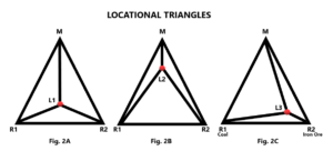
Cases in Location Triangles
Fig. 2 shows three scenarios where there are two raw materials and one market. There may be more raw materials in the real situation but the logic will remain same for selecting location.
- In the first case (Fig. 2A), both the raw materials at R1 & R2 are weight losing. Therefore, the producer locates his industry at L1. Eventually, the producer has to transport a lighter product to the market and the total cost will be lesser.
- In the second case (Fig. 2B), both the raw materials are weight gaining. It means that the weight of the final product becomes greater than the weight of two raw materials. Therefore, it is wise to transport these raw materials close to market before making the final product. This way, the producer can save the additional transport which he might incur if he located his firm near the source of raw materials.
- In the third case (Fig. 2C), the raw materials are weight losing. Hence, the final product is lighter than the weight of raw materials. However, the producer has to use one raw material (R2) more than the other (R1). So, it would be profitable to locate the industry near R2 because R2 is used in higher quantities than the R1. Let us clarify with the help of an example. A producer needs 4 quintals of iron ore and 2 quintals of coking coal for producing 1 quintal of pure iron. In this case, it would be economic to transport the 2 quintals of coking coal to R2 rather than transporting 4 quintals of iron ore to R1. Therefore, the producer will locate the industry near R2 rather than the R1 because the cost of transporting 4 quintals of iron ore is greater than 2 quintals of coal.
- Material Index: In short, Weber opined that the material index determines whether the industry will locate at source or at market. The goods having material index greater than one will try to locate at source while the goods with less than one will try to locate at market. The formulae for material index is as follows.
Material Index (MI) = Weight of Raw Material ÷ Weight of Finished Product
2. Influence of Labor Cost
Weber assumed that labor supply in different locations is constant but their wages vary. The variation in wage rate influences the industrial location, too. The producer will be ready to locate his firm at a location other than the location of least transport cost, when the decline in wages will be offset by the increase in transport cost.
- Take the example of the iron and steel industry. In Fig. 2C, the producer locates his industry at L3 near R2 to avoid extra transport cost. However, if we take the labor cost into consideration, the producer may consider a different location than L3.
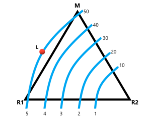
- Let us understand “why the producer will consider another location?” In Fig. 3, blue lines are isotims. The isotims are the lines which join the areas of equal additional transport cost from a given point.
- In Fig. 3, blue lines join the areas of equal transport cost from R2. The iron and steel industry is located at R2. The cost of production is as follows.
- Suppose, the total cost of transportation of raw materials from mines and final product to the market is 400 per unit.
- The labor cost for the production process is 250 per unit.
- Total cost is 400 + 250 = 650.
- It is observable in Fig. 3 that the additional transport cost at 5th isotim is Rs. 50 more than the location near R2.
- However, if the labor cost is Rs. 100 per unit at 5th isotim, the total cost will be sum of the transport cost, additional transport cost and total labor cost i.e. 400 + 50 + 100 = Rs. 550.
- Thus, it will be economic and profitable to locate the industry at point ‘L’ on the 5th isotim
3. Influence of Agglomeration
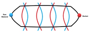
Weber also tried to demonstrate the impact of industrial agglomeration on the location of industry through Isodapane. Isodapane refers to the line joining the areas of equal total cost i.e. sum of transport and labour cost (Fig. 4). The total transport cost includes the cost of transporting raw material from its source and the cost of transporting the final product to the market from the factory. In fig. 4, the red lines are isotims from the market and blue lines are isotims from the source of raw material. The total cost is equal at the intersection of blue and red isotims. The black line joins these intersecting points of equal total cost. This black line is isodapane (Fig. 4).
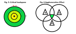
Critical Isodapane and Agglomeration Effect
- A producer can locate his factory up to a point where the increase in total transport cost is offset by decline in labour cost. In Fig. 5. The 1, 2 and 3 are isodapanes showing additional total transportation cost of Rs. 5, 10 and 15, respectively. At location ‘L1’ in Fig. 5, the labor cost is Rs.15 cheaper than the location of least transport cost i.e. the center of the circle. However, the additional total transport cost at L1 is Rs. 15 more. Therefore, the labor cost offsets additional transport cost. In this case 3rd Isodapane is the Critical Isodapane.
- The agglomeration refers to the location of many firms and industries close to each other at an economically favorable place e.g. in large cities, near ports, near railway junctions etc. The agglomerations are like Growth Poles and there are many benefits and externalities of locating a firm or factory at industrial agglomeration. The cost of labor, raw materials, technology and transport is low at industrial agglomeration. Therefore, the margin for profit is greater. Read Myrdal’s Cumulative Causation Theory and Hirschman’s Unbalanced Growth Theory for details of impact of agglomeration on economy.
- Weber combined the impact of labor cost, transport cost and the agglomeration effect (see Fig. 6) to demonstrate a holistic view of the industrial location. He drew critical isodapanes around three locations of least transport cost. These isodapanes overlap over a small area. This overlapping area has been shaded green in Fig. 6. It will be economical for the firms to locate their industries in this green area because the increase in total transport cost is offset by the decline in labor cost within this area. Additionally, all these three industries can operate in coordination which can reduce transport and input costs.
Conclusion
In short, we can argue that industrial location theory tries to maximize the profit of firms by suggesting a location of least transport cost. However in certain conditions where labor cost offsets the increased transport cost, the producer may locate away from the location of least transport cost. Above all, the agglomeration of industries takes place where the critical isodapanes of multiple locations overlap. Such agglomerations help in quick access to new technology, transportation facilities, cheap labor etc. Finally, we can argue that the optimum location of industries may differ from location of least transport cost but only when the decline in other costs outweigh the increase in transport cost.
Kulwinder Singh is an alumni of Jawaharlal Nehru University, New Delhi and working as Assistant Professor of Geography at Pt. C.L.S. Government College, Kurukshetra University. He is a passionate teacher and avid learner.